Using a Spreadsheet to Organize Data,

Calculate the Hours of Daylight in Washington, D.C. and Make a Graph

1. Open ClarisWorks and select Word Processing.
2. Make the tools available. (View/Show tools.)
3. Select the Spreadsheet tool and click and drag to make a spreadsheet with 13 rows and 4 columns.
4. Type in the column headings. You can center the headings by:
   • Highlight all the headings.
   • Then from the menu bar, click on Format and drag to Alignment and then Center.

   

5. Type in the months of the year. Use three-letter abbreviations for the names of the months.
   
6. Before typing in the data for sunrise and sunset, format the cells for numbers by:
   • Highlight the columns for sunrise and sunset.
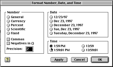
   • From the menu bar click on Format and drag to number
   • Click in the box shown below.

   

    

7. Type in the data for sunrise and sunset. For example: For JAN Type 7:23 for sunrise and press return. The computer will add the AM. For sunset, type 17:17 and press return. The computer will enter 5:17 PM in the cell.

   
    

8. To calculate the number of hours of daylight in Washington, D.C. for the 21st of each month, subtract the time of sunrise from the time of sunset.
   The number of hours of daylight is also referred to as the duration of insolation (insolation stands for incoming solar radiation). Remember, before subtracting using pencil and paper, times should be expressed in 24-hour format. You can change the times in your spreadsheet to the 24-hour format by highlighting columns C and D and selecting the 24-hour format as described in the next step.
   
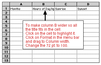
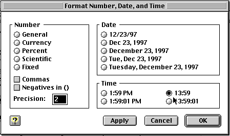
9. One of the great things about a spreadsheet is it can DO MATH. Before typing the formula, highlight column B. From the menu bar, click on Format and drag to Number. This time select the 24-hour format as shown below.
   
10. To have the computer calculate the hours of daylight type the formula in the entry bar.
    • Click in the cell A2, Hours of Daylight for JAN.
    • Type an equal sign. All formulas begin with the equal sign.
    • Then click in cell D2 (Sunset for JAN). You will notice in the entry bar D2 now follows the equal sign.
    • Next type a minus sign in the entry bar.
    • Click in cell C2.
    • The entry bar should look as follows:
      
    • When you press return the answer should appear in cell A2. 9:54 means 9 hours 54 minutes.
11. To make your graph:
    • Highlight all of your data in the column A and B, including the column headings.
    • Click on Options in the menu bar and drag to Make chart.
    • Select line graph and click OK.